|
|
|
|
|
|
There are two main data types: a list of miRNAs, miR-SNPs, genes, small molecules, etc.; or a data table from qPCR, microarray or RNAseq for mRNA or miRNA experiments. The list data is a list of IDs with optional fold change values. The expression data is a table in tab delimited text file format with miRNAs/gene IDs in rows and samples in columns. The first column is for gene or probe IDs. The following common ID types are supported:
miRNA sequence domains are defined as primary (100 bp sequence flanking the precursor – "Primary‐Up" and "Primary‐Down"), 5′ and 3′ precursor arms ("End"), 5′ and 3′ mature, seed region (2–8 bp of mature miRNA), and precursor loop (between mature miRNA) according to Oak,et.al.,(2019).
In the study of Shu,et.al.,(2016), to characterize the potential deciding features of transportable microRNAs, specifically, they analyzed all publicly available microRNAs, a total of 34,612 from 194 species, with 1,102 features derived from the microRNA sequence and structure. And ranking them by the transportable probability. In the Xeno-miRNet, we selected top 3000 miRNAs from their results and overlaped the xeno-species with the detected data.
Including the predicted transportable miRNAs may return a very large data. Users can try not to include them at the first time, and if the data size is reasonable, users can include the predicted miRNAs later.
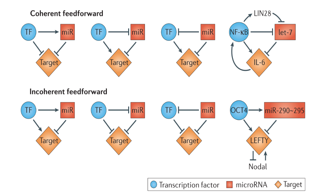
In transcription factor (TF)-miRNA feed-forward loops, TF and miRNA co-regulate the target genes. Specifically, feed-forward loops are classified into coherent and incoherent loops as illustrated in the figure below from Bracken, et al. 2016.
#NAME           Sample1	Sample2	Sample3	Sample4	Sample5	Sample6	Sample7	Sample8 Sample9
#CLASS  	Y   	N	N	Y	N	Y	Y	N       N
100_g_at        -3.06	-2.25	-1.15	-6.64	0.4	1.08	1.22	1.02    1.15
1000_at         -1.36	-0.67	-0.17	-0.97	-2.32	-5.06	0.28	1.32    0.73
1002_f_at       1.61	-0.27	0.71	-0.62	0.14		0.11	0.98    0.54
1008_f_at       0.93	1.29	-0.23	-0.74	-2	-1.25	1.07	1.27    1.02
You can choose to use our example datasets for your testing. Example microarray gene expression data from eight Affymetrix Human Genome U95 chips (hgu95av2)
can be downloaded here for testing.
Microarray data provides probe-level expression measurements, while RNA-seq data provides expression at exon-level or transcript-level (i.e. different isoforms of the same gene) expression measurements. However, current functional annotations are assigned at the gene level. It is necessary to first map the probe-level or transcript-level measurements to the corresponding gene-level measurements.
When multiple probes or transcripts are mapped to the same gene, they need to be summarized into a single value for the corresponding gene. In miRNet, the averages of multiple probe intensities (microarray/QPCR), or sums of counts from multiple transcripts (RNAseq) are used to perform gene-level summarization.
If the data is not already normalized, you need to choose a proper method for data normalization. It is generally considered that differences in expression exist on a multiplicative scale. For microarray data analysis using linear model (limma), log transformation should be used to bring them into the additive scale, where a linear model may apply. For RNAseq data analysis using edgeR, the Trimmed Mean of M values (TMM) should be used. Many common normalization methods have been offered for QPCR data normalization. Point the mouse to the help icon on the normalization section to find more about each normalization procedure.
If you are not sure whether the data is already log transformed or not, you can easily figure this out by visualizing the data (i.e. boxplot). For microarray data, log transformed data values are usually less than 16. For count data with 1 million counts, log2(1,000,000) is less than 20. Therefore, if all data values are below 20, it is reasonable to assume that the data has already been log transformed.
There have been significant changes and updates in the miRNA naming conventions over the past decade. As a result, many miRNA annotations and IDs are not valid any more. The miRNet functional annotations and associations are based on miRNA IDs and Accessions of the current miRBase (version 22). We strongly recommend you to double check and update your miRNA IDs against the current miRBase if there are no hits found for you input.
If you are doing miRNA expression analysis, you can analyze the data first to identify significant miRNAs and then manually updates the IDs for those miRNAs. The updated miRNAs can be copy-and-paste as a list for network analysis and interpretation using miRNet.
Yes, this task can be achieved using the Data Filter dialog on the Interaction Table page. On the page, click the Data Filter button to bring up the dialog. On the list of methods, select those methods you want to include and click OK. The Interaction table will be filtered to contain only those validated by the selected approaches. Note, for S.mansoni where only predicted interactions are available, you can select a threshold of the score to control the confidence level.
Yes, miRNet provides multiple functions to help with this task. First go to the Interaction Table page:
Too many nodes will make the network too dense to visualize and the computer slow to respond. We recommend limiting the total number of nodes to between 200 ~ 2000 for the best experience. We provide several Network Tools to help deal with network size when the networks are too large and complex to be visualized or interpreted. The basic idea is to focus only on those nodes that are more likely to be "important" as measured by their centrality within the network (see the previous FAQ for more details).
The "Shortest Path Filter" is designed to reduce the "hair-ball" effect in the network visualization. The goal is to extract a minimally connected subgraph, by computing pair-wise shortest paths between all major hub nodes, and then remove the nodes that are not on the shortest paths.
Yes. You can use the Batch Filter under the Network Tools to enter a list of molecules. These molecules together with your query list will be used to filter the network. At the moment, the function only support the miRNA-target gene interaction network
Both the Minimum Network and Steiner Forest Network tools aim to construct a minimally connected network that contains all of the seed genes. This means that the only added nodes are ones that connect previously disjointed networks of seed genes. The difference between the minimum network and the Steiner forest network is the way in which the approximate solution is computed. For the minimum network, miRNet implements an approximate approach based on shortest paths: we compute pair-wise shortest paths between all seed nodes, and remove the nodes that are not on the shortest paths. For the Steiner forest network, miRNet implements a fast heuristic Prize-collecting Steiner Forest algorithm.
|
Important nodes can be identified based on their position within the network. The assumption is that changes in the key positions within a network will have more impact on the network than changes at the periphral or relatively isolated positions. miRNet provides two well-established node centrality measures to estimate node importance - degree centrality and betweenness centrality. In a graph network, the degree of a node is the number of connections it has to other nodes. Nodes with higher node degree act as hubs in a network. The betweenness centrality measures the number of shortest paths going through the node. It takes into consideration the global network structure. For example, nodes that occur between two dense clusters will have a high betweenness centrality even if their degree centrality values are not high. Note, you can sort the node table based on either degree or betweenness values by double clicking the corresponding column header. |
The nodes from input list (seed nodes) will be marked as asterisk symbol (*) in the Node Explorer.
To highlight seed nodes, please click on highlight seed nodes icon ![]() located
in the vertical tool bar on the top left corner of Network Viewer.
located
in the vertical tool bar on the top left corner of Network Viewer.
Please use the Download option and choose "SVG Format" to save the current network view (use Chrome or FireFox, known issue with Safari). SVG is a vector based graphic format and you can then export it into any resolution static image (i.e. png) using a suitable graphic tool, for example, the powerful free tool InkScape. Note, it is best to save SVG in white background, as the default background color in InkScape is in white. If your SVG is saved in Black background, after opening the SVG in InkScape, set the Background color to black (hex code: #222222) using the Document Properties menu.
Yes. miRNet supports black (default), white and customized background. To switch background color, click the pull-down menu next to Background on the toolbar at the top of the screen. From the dropdown menu list, select a color.
You can change the color, size, and shape of a node. To change the node color, you need to first choose the color using the Color Palette for the next selection, then select (by clicking on the node) you want to change. The node color will be changed to your specification. To change node size, you can keep clicking it (double-clicking) to increase its size. You can also use the Node Size functions to increase or decrease the node size. To change node shape, you need to first choose "All nodes" or "Highlighted nodes", then select the shape you want to change.
Yes. By default, you can drag and drop to change position of a single node - simply put your mouse cursor over the node. When its label shows up, left click and drag the node to a position. Release the mouse. To change positions for multiple nodes, there are several built-in approaches. First use the Scope option on the top menu bar to make sure that the option Node-neighbours is selected. Then drag the central node of the node cluster to a new position. Note, only dependent nodes (nodes that are only connected with the central node, but not to any other nodes) will be affected. If you also want to adjust the position of these non-dependent nodes, switch the Scope to Single node, and then drag these nodes individually to the new position. You can manually select multiple nodes using Manual seleciton and then drag them together to new positions.
Nodes will be automatically labeled when their sizes reach a certain threshold. Therefore, you can simply increase node size to label any node. To do so:
Yes, miRNet currently supports seven types of network layout, including Force Atlas, Fruchterman-Reingold, Graphopt, Large Graph, Random, Reduce Overlap, Bipartite and Tripartite layout.
There are two basic steps in the network highlighting - setting the highlight color and making selections. Use the Color Palette to set the color for the Next selection.
 , when mouse icon becomes cross hair, drag to select;
Yes. First select the miRNAs/genes of interest uisng the checkboxes in the node table on the left panel; Locate the "Highlight shared/all interactions" function on the table tool bar; Choose "Shared" instead of the default "All" option; Click "Submit" button. The shared nodes, the source nodes as well as their connections will be highlighted on the network. You can then perform enrichment analysis on these shared genes.
Yes. To do this, first select or highlight section of the network, then click the
Extract  icon on the left tool bar in the network view window.
Yes, after you have performed functional enrichment analysis the over-represented themes will be displayed in the table below. By double clicking on a pathway name, all gene members of the pathway will be highlighted nodes within the current network with large size and colored based on current color choice.
The enrichment analysis is to test whether any functional modules (gene sets) from the user selected library are significantly enriched among those genes of interest (i.e. if a particular group of gene funciton is more frequently observed than would be anticipated by random chance). miRNet offers the standard enrichment analysis based on the hypergeometric tests after adjustment for false discovery rate (FDR). However, for those genes are identified from the miRNA target analysis (i.e. the input is miRNA), the assumption of random sampling of the "gene universe" is not valid and the standard approach could be biased (refer to the paper Bias in microRNA functional enrichment analysis for more details). Note, the enrichment analysis result can be downloaded from Download menu.
The unbiased empirical sampling method is used to estimate the null distribution of the target genes as selected based on the input miRNAs. The procedures can be devided into three steps: 1) A list of miRNAs of the same size are randomly selected from all the miRNAs with known targets in the database; 2) The functional annotations (i.e. GO or KEGG) are then performed for the list; 3) The process is repeated 1000 times (default); 4) Compare the hits in each GO or KEGG pathways and the empirical p (Emp. p) values are calculated as the proportion of overlaps (with pathways or GO) from 1000 random process that equal or larger than the original. A p value < 0.001 will be reported if no results from random process are better than the original.
Yes, miRNet currently supports nine different databases for functional enrichment analysis, including:
Yes, as limited by the public server, each computing is 1000 random samplings. However, the computed results are saved. If user click to perform the functional analysis again under the same parameters, the results will be combined. i.e. clicking five times will generate empirical p values based on 5000 random samplings.
Yes. Users can perform enrichment tests on currently highlighted nodes in the network. To highlight nodes of interest, there are two basic approaches:
Modules are tightly clustered subnetworks with more internal connections than expected randomly in the whole network. They are considered as to be relatively independent components in a graph. Members within a module are likely to work collectively to perform a biological function. The biological functions of a module can be explored using enrichment analysis.
miRNet currently offers three different approaches for module detection - the WalkTrap, InfoMap, and Label Propagation algorithms. The general idea behind the Walktrap Algorithm is that if you perform random walks on a graph, a higher number of walks are more likely to stay within a group of nodes that are highly connected to each other because there are only a few edges that lead outside of them. The Walktrap algorithm runs many short random walks and uses the results to detect small modules, and then merge separate smaller modules in a bottom-up manner. The InfoMap Algorithm is also based on random walks, which it uses to minimize the hierarchical map equation for different partitions of the network into modules. The Label Propagation Algorithm works by randomly assigning a unique label to every node. On each iteration, node labels are updated to match the one that the maximum of its neighbours has. The algorithm converges when each node has the same label as the majority of its neighbours.
The p-value of a module is based solely on network connectivity, and gives some indication of how significant the connections within a defined module are. Let's call the edges within a module "internal" and the edges connecting the nodes of a module with the rest of the graph "external". The null hypothesis of the test is that there is no difference between the number of "internal" and "external" connections to a given node in the module. The p-value of a given module is calculated using a Wilcoxon rank-sum test of the "internal" and "external" degrees. Users should also consider whether the modules are 'active' under the experimental conditions, by taking into account the number of seeds, their average fold changes (gene expression), as well as the enriched functions displayed in the Module Explorer table.
